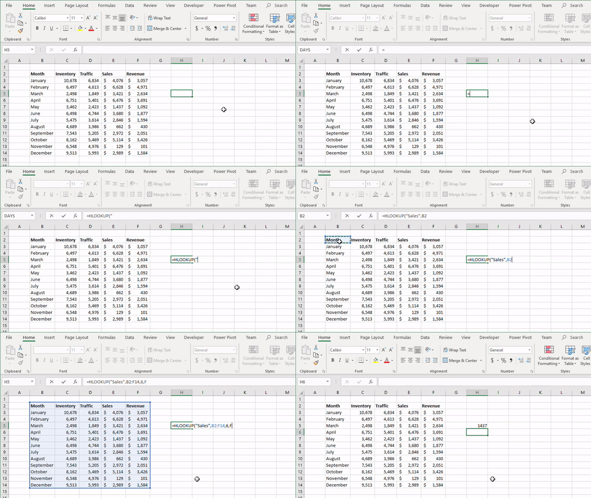
The HLOOKUP function

The HLOOKUP function is a lookup and reference function which allows you to search for a value in the first row of a selected range, and return the value from the appropriate column the designated number of rows down the range. It is the sister function to VLOOKUP, which performs the same operation on the opposite axis.

This is the format of the HLOOKUP function:

=HLOOKUP(LOOKUP VALUE, LOOKUP RANGE, ROW INDEX NUMBER, EXACT MATCH)

Here is an example of the HLOOKUP function:

=HLOOKUP(“Sales”, A1:G10,6,FALSE) = D6 (When “Sales” is in cell D1) 

HLOOKUP function returning the sixth row of the sales column from the table

This function is valuable when your primary search drivers are located as headers to your data set. Normally this would be used when you know in which row your result should be in, but not where the value you are searching for would be.

An example of a functional implementation of this would be when you have a weekly reporting sheet that tracks a variety of metrics week over week. Along row 4 you have the fiscal week number associated to the data. You know the metric you are trying to analyze sits in row 7, and now you need to consolidate the data from specific weeks onto another sheet.

=HLOOKUP(WEEK NUMBER, 4:7, 4, FALSE)